Introducing the schrute Package: the Entire Transcripts From The Office

I’m going to Costa Rica

LinkedIn | Github | Blog | Subscribe

What

This is a package that does/has only one thing: the complete transcriptions of all episodes of The Office! (US version). Schrute package website

Use this data set to master NLP or text analysis. Let’s scratch the surface of the subject with a few examples from the excellent Text Mining with R book, by Julia Silge and David Robinson.

First install the package from CRAN:

# install.packages("schrute")
library(schrute)
library(dplyr)

Attaching package: 'dplyr'

The following objects are masked from 'package:stats':

    filter, lag

The following objects are masked from 'package:base':

    intersect, setdiff, setequal, union

There is only one data set with the schrute package; assign it to a variable

mydata <- schrute::theoffice

Take a peek at the format:

dplyr::glimpse(mydata)

Rows: 55,130
Columns: 12
$ index            <int> 1, 2, 3, 4, 5, 6, 7, 8, 9, 10, 11, 12, 13, 14, 15, 16…
$ season           <int> 1, 1, 1, 1, 1, 1, 1, 1, 1, 1, 1, 1, 1, 1, 1, 1, 1, 1,…
$ episode          <int> 1, 1, 1, 1, 1, 1, 1, 1, 1, 1, 1, 1, 1, 1, 1, 1, 1, 1,…
$ episode_name     <chr> "Pilot", "Pilot", "Pilot", "Pilot", "Pilot", "Pilot",…
$ director         <chr> "Ken Kwapis", "Ken Kwapis", "Ken Kwapis", "Ken Kwapis…
$ writer           <chr> "Ricky Gervais;Stephen Merchant;Greg Daniels", "Ricky…
$ character        <chr> "Michael", "Jim", "Michael", "Jim", "Michael", "Micha…
$ text             <chr> "All right Jim. Your quarterlies look very good. How …
$ text_w_direction <chr> "All right Jim. Your quarterlies look very good. How …
$ imdb_rating      <dbl> 7.6, 7.6, 7.6, 7.6, 7.6, 7.6, 7.6, 7.6, 7.6, 7.6, 7.6…
$ total_votes      <int> 3706, 3706, 3706, 3706, 3706, 3706, 3706, 3706, 3706,…
$ air_date         <chr> "2005-03-24", "2005-03-24", "2005-03-24", "2005-03-24…

 mydata %>%
  dplyr::filter(season == '01') %>%
  dplyr::filter(episode == '01') %>%
  dplyr::slice(1:3) %>%
  knitr::kable()

index	season	episode	episode_name	director	writer	character	text	text_w_direction	imdb_rating	total_votes	air_date

So what we have is the season, episode number and name, character, the line spoken and the line spoken with the stage direction (cue).

We can tokenize all of the lines with a few lines from the tidytext package:

token.mydata <- mydata %>%
  tidytext::unnest_tokens(word, text)

This increases our data set to 571612 records, where each record contains a word from the script.

 token.mydata %>%
  dplyr::filter(season == '01') %>%
  dplyr::filter(episode == '01') %>%
  dplyr::slice(1:3) %>%
  knitr::kable()

index	season	episode	episode_name	director	writer	character	text_w_direction	imdb_rating	total_votes	air_date	word

If we want to analyze the entire data set, we need to remove some stop words first:

stop_words <- tidytext::stop_words

tidy.token.mydata <- token.mydata %>%
  dplyr::anti_join(stop_words, by = "word")

And then see what the most common words are:

tidy.token.mydata %>%
  dplyr::count(word, sort = TRUE) 

# A tibble: 18,960 × 2
   word        n
   <chr>   <int>
 1 yeah     2930
 2 hey      2232
 3 michael  1860
 4 uh       1463
 5 gonna    1405
 6 dwight   1345
 7 jim      1162
 8 time     1149
 9 pam      1043
10 guys      947
# ℹ 18,950 more rows

tidy.token.mydata %>%
  dplyr::count(word, sort = TRUE) %>%
  dplyr::filter(n > 400) %>%
  dplyr::mutate(word = stats::reorder(word, n)) %>%
  ggplot2::ggplot(ggplot2::aes(word, n)) +
  ggplot2::geom_col() +
  ggplot2::xlab(NULL) +
  ggplot2::coord_flip() +
  ggplot2::theme_minimal()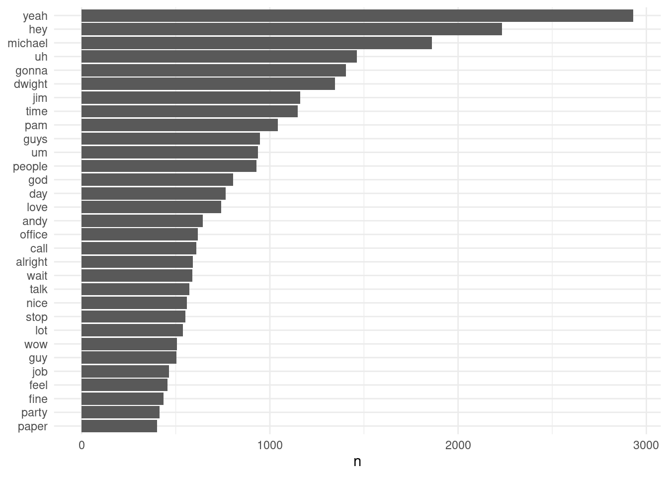

Feel free to keep going with this. Now that you have the time line (episode, season) and the character for each line and word in the series, you can perform an unlimited number of analyses. Some ideas: - Sentiment by character - Sentiment by character by season - Narcissism by season (ahem.. Nard Dog season 8-9) - Lines by character - Etc.

---

Want more content like this? Subscribe here